Programming with R: Challenges

Introduction to RStudio

Challenge 1

Which of the following are valid R variable names?

min_height
max.height
_age
.mass
MaxLength
min-length
2widths
celsius2kelvin

Challenge 2

What will be the value of each variable after each statement in the following program?

mass <- 47.5
age <- 122
mass <- mass * 2.3
age <- age - 20

Challenge 3

Run the code from the previous challenge, and write a command to compare mass to age. Is mass larger than age?

Seeking Help

Challenge 1

Look at the help for the c function. What kind of vector do you expect you will create if you evaluate the following:

c(1, 2, 3)
c('d', 'e', 'f')
c(1, 2, 'f')`

Challenge 2

Look at the help for the paste function. You’ll need to use this later. What is the difference between the sep and collapse arguments?

Challenge 3

Use help to find a function (and its associated parameters) that you could use to load data from a csv file in which columns are delimited with “\t” (tab) and the decimal point is a “.” (period). This check for decimal separator is important, especially if you are working with international colleagues, because different countries have different conventions for the decimal point (i.e. comma vs period). hint: use ??csv to lookup csv related functions.

Data Structures

Challenge 1

Predict what will happen if we perform an operation between two vectors of different size?

Test your guess by creating two vectors of different lengths using the colon operator and adding or multiplying them together.

Challenge 2

What happens when we create a vector that combines data types?

Try creating a vector named my_vector containing the elements 1, “four”, and TRUE. What does the vector look like?

Use the str command to determine what data type is in your vector?

Challenge 3

R also vectorizes functions on character vectors as well.

Use the c function to create a character vector named colors with the values: “red”, “yellow” and “blue”. Use the paste function to combine "My ball is" with each element of your vector.

Subsetting Data

Challenge 1

Given the following code:

x <- c(5.4, 6.2, 7.1, 4.8, 7.5)
names(x) <- c('a', 'b', 'c', 'd', 'e')
print(x)

  a   b   c   d   e
5.4 6.2 7.1 4.8 7.5

Come up with at least 2 different commands that will produce the following output:

  b   c   d
6.2 7.1 4.8

After you find 2 different commands, compare notes with your neighbour. Did you have different strategies?

Challenge 2

Run the following code to define vector x as above:

x <- c(5.4, 6.2, 7.1, 4.8, 7.5)
names(x) <- c('a', 'b', 'c', 'd', 'e')
print(x)

  a   b   c   d   e
5.4 6.2 7.1 4.8 7.5

Given this vector x, what would you expect the following to do?

x[-which(names(x) == "c")]

Test out your guess by trying out this command. Did this match your expectation? Why did we get this result? (Tip: test out each function in the order it’s applied—this is a useful debugging strategy.)

Challenge 3

While it is not recommended, it is possible for multiple elements in a vector to have the same name. Consider this example:

y <- 1:3
y

[1] 1 2 3

names(y) <- c('a', 'a', 'a')
y

a a a
1 2 3

Using named subsetting can you come up with a command that will return only one of the 'a' values and a different command that will return all of the 'a' values? Does your answer differ from your neighbors?

Challenge 4

Given the following code:

x <- c(5.4, 6.2, 7.1, 4.8, 7.5)
names(x) <- c('a', 'b', 'c', 'd', 'e')
print(x)

  a   b   c   d   e
5.4 6.2 7.1 4.8 7.5

Write a subsetting command to return the values in x that are greater than 4 and less than 7.

Exploring Data Frames

Challenge 1

There are several subtly different ways to call variables, observations and elements from data.frames:

• cats[1]
• cats$coat
• cats[“coat”]
• cats[1, 1]
• cats[, 1]
• cats[1, ]

Try out these examples and explain what is returned by each one.

Challenge 2

Remember that you can create a new data.frame right from within R with the following syntax:

variable1 <- c('a', 'b', 'c')
variable2 <- c(1, 2, 3)
variable3 <- c(TRUE, TRUE, FALSE)
df <- data.frame(variable1,
                 variable2,
                 variable3,
                 stringsAsFactors = FALSE)

Note that the stringsAsFactors setting allows us to tell R that we want to preserve our character fields and not have R convert them to factors.

Modifying the syntax above, make a data.frame that holds the following information for yourself:

• first name
• last name
• lucky number

Then use rbind to add an entry for the people sitting beside you. Finally, use cbind to add a column with each person’s answer to the question, “Is it time for coffee break?”

Challenge 3

Fix each of the following common data frame subsetting errors:

1. Extract observations collected for the year 1957.

   gapminder[gapminder$year = 1957,]
   

2. Extract all columns except 1 through 4.

   gapminder[,-1:4]
   

3. Extract the rows where the life expectancy is longer than 80 years.

   gapminder[gapminder$lifeExp > 80]
   

4. Extract the first row, and the fourth and fifth columns (lifeExp and gdpPercap).

   gapminder[1, 4, 5]
   

5. Advanced: extract rows that contain information for the years 2002 and 2007.

   gapminder[gapminder$year == 2002 | 2007,]
   

Challenge 4

1. Why does gapminder[1:20] return an error? How does it differ from gapminder[1:20, ]?

2. Create a new data.frame called gapminder_small that only contains rows 1 through 9 and 19 through 23. You can do this in one or two steps.

Control Flow

Challenge 1

Use an if statement to print a suitable message reporting whether there are any records from 2002 in the gapminder dataset. Then write a similar statement that reports if there are both 2002 and 2012 records.

Challenge 2

Write a script that loops through the gapminder data by continent and prints out the continent, the mean life expectancy on that continent, and whether or not that life expectancy is larger than 65 years. Hint: If x is a numeric vector, mean(x) returns the mean of x. For any vector x, unique(x) returns a vector with the unique values of x. Finally cat("x is",6) prints x is 6.

Challenge 3

Modify the script from Challenge 4 to loop over each country. This time print out whether the life expectancy is smaller than 50, between 50 and 70, or greater than 70.

Dataframe Manipulation

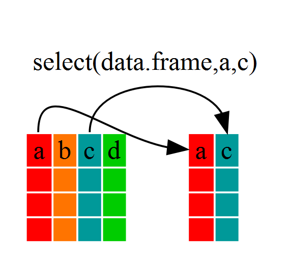
Challenge 1

Write a single command (which can span multiple lines and includes pipes) that will produce a data frame that has the African values for lifeExp, country and year, but not for other continents. How many rows does your dataframe have?

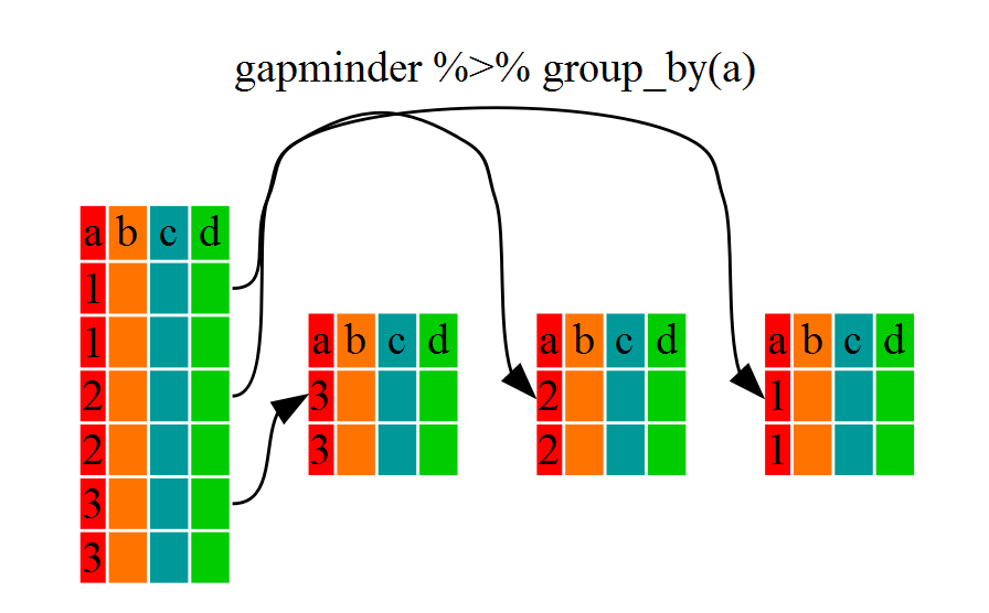
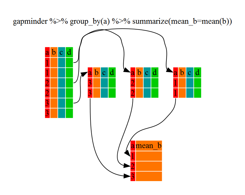
Challenge 2

Calculate the average life expectancy per country. What is the longest average life expectancy and the shortest life expectancy?

Challenge 3

Calculate the average life expectancy in 2002 for each continent.

Challenge 4 - Advanced

Modify your code from Challenge 3 to randomly select 2 countries from each continent before calculating the average life expectancy and then arrange the continent names in reverse order.

Hint: Use the dplyr functions arrange and sample_n. They have similar syntax to other dplyr functions. Be sure to check out the help documentation for the new functions by typing ?arrange or ?sample_n if you run into difficulties.

Creating Publication Quality Graphics

Challenge 1

Our example visualizes how the GDP per capita changes in relationship to life expectancy:

ggplot(data = gapminder, aes(x = gdpPercap, y = lifeExp)) + geom_point()

Modify this example so that the plot visualizes how life expectancy has changed over time:

Hint: the gapminder dataset has a column called year, which should appear on the x-axis.

Challenge 2

In the previous examples and challenge we’ve used the aes function to tell the scatterplot geom about the x and y locations of each point. Another aesthetic property we can modify is the point color. Modify the code from the previous challenge to color the points by the continent column. What trends do you see in the data? Are they what you expected? Hint: There’s more than one way to do this. One approach is to view color as an aesthetic property of the point (geom_point). Try executing ?geom_point and looking under both Aesthetics and Examples.

Challenge 3

Modify the color and size of the points on the point layer in the last example (not the last challenge).

Hint: do not use the aes function. Rather add arguments to the correct function.

Challenge 4

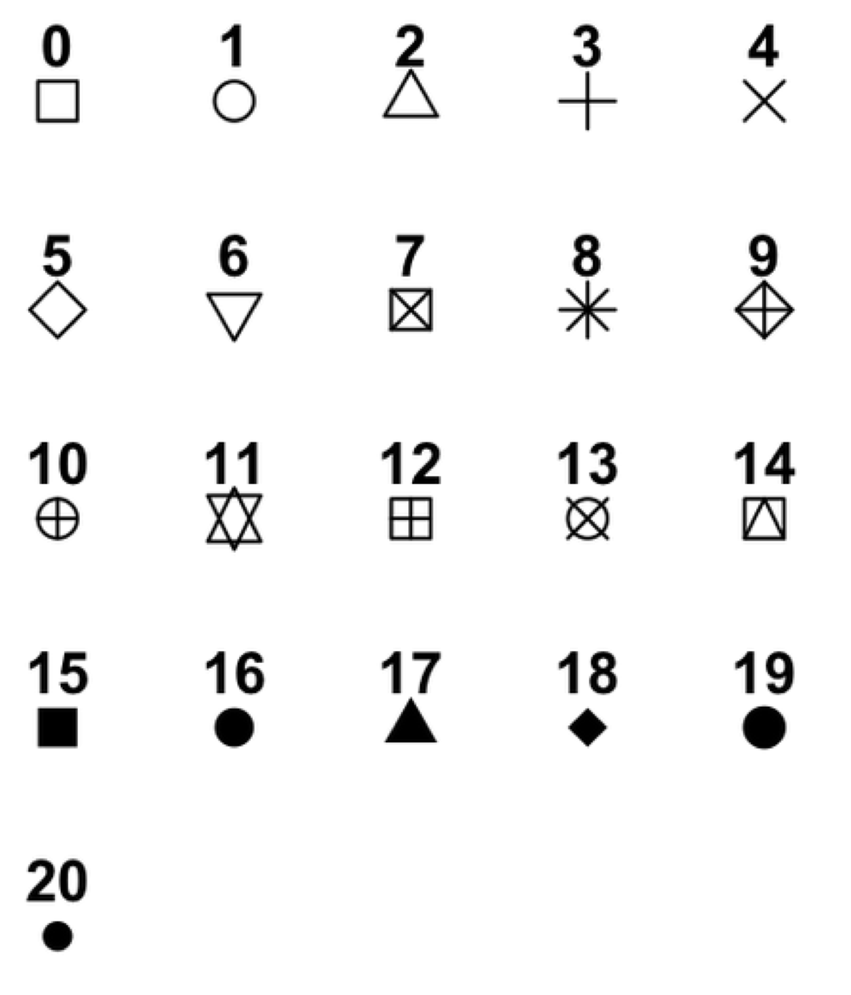
Modify your solution to Challenge 3 so that the points are now a different shape and are colored by continent with one least-squares trendline per continent.

Hint: The color argument should be used inside aes inside ggplot. To change the shape of a point, use the pch argument within geom_point. Setting pch to different numeric values from 1:25 yields different shapes as indicated in the chart below:

Writing Data

Challenge 1

Write a data-cleaning script file that subsets the gapminder data to include only data points collected since 1990.

Use this script to write out the new subset to a file your working directory.

Remember to use a different file name so that the new output doesn’t overwrite your old output.

Wrapup

If you want to learn more, check out some of these great resources:

Help Files in R

Don’t forget your R helpfiles and package vignettes which can be accessed by using the ? and vignette commands.

Workshop Lessons

These are the lessons used in the workshop with solutions for challenges.

Supplemental Lessons

Additional R topics that we could not cover today.

RStudio cheat sheets

R quick reference guides including today’s handouts and more!

R for Data Science

Hadley Wickham is RStudio’s Chief Data Scientist and developer of the dplyr and ggplot2 packages. R for Data Science is his newest book, and is available here for free.

One R Tip a Day on Twitter

Following One R Tip a Day is a great way to learn new tips and tricks in R.

Twotorials

Twotorials is a compilation of 2 minute youtube videos which highlight a specific topic in R.

Quick R Website

Cookbook for R

Advanced R

For more advanced topics, check out Hadley Wickham’s website based on his book “Advanced R”.