Programming with R: Guide
Day 1: Thursday, Feb. 15, 2018
Introduction to R and RStudio: 1:00–1:30
Before Starting The Workshop
On artin, as nelle:
$ rm ~/swc/2018-02-15-earlham-owm/earlham.R
$ touch ~/swc/2018-02-15-earlham-owm/earlham.R
$ cd ~/swc/earlham-notes
$ gitautopush ../2018-02-15-earlham-owm/earlham.R
Please ensure you have the latest version of R and RStudio installed on your
machine. Browser tabs: workshop, etherpad, bit.ly/earlham-R and
bit.ly/earlham-notes.
Note to self: don’t create new values for variables as it will affect future evaluations in your script. You can make a copy of a variable, however.
Introduction to RStudio
Why R?
- free
- open source
- statistics, rather than general-purpose
- statistical pkgs created by statisticians.
Why RStudio?
- provides a fully integrated environment
- built in version control and project management
- works on all platforms
Goal: learn enough R to understand Stack Overflow answers for basic R programming questions.
Basic layout
Type along with me. If you fall behind, check bit.ly/earlham-notes or the
etherpad.
Three panels:
- The interactive R console (entire left)
- Environment/History (tabbed in upper right)
- Files/Plots/Packages/Help/Viewer (tabbed in lower right)
Editor panel appears when you open scripts.
Work flow within RStudio
There are two main ways one can work within RStudio.
- Test and play within the interactive R console then copy code into
a
.Rfile to run later. - Start writing in a
.Rfile and use RStudio’s command/shortcut to push current line, selected lines or modified lines to the interactive R console.
We’ll do the latter (as do I when I write my R scripts).
Start with File->New File->R Script. Use getwd() to find out where you are
and save this somewhere. Use Save As to name your file, e.g. swc.R.
Run button and key shortcuts
- Ctrl-enter windows/linux
- Command-enter mac
Mostly use the console to run code and test commands.
In the console, the > prompt is similar to the shell’s $ prompt. There
you can
- Type commands.
- R executes them &
- R returns result
1:07 The simplest thing you can do with R is arithmetic:
1 + 100
Ignore the [1] for now.
Demo bit.ly/earlham-notes.
Incomplete commands:
> 1 +
Can cancel with the “Esc” key.
Order of operations:
3 + 5 * 2
Use parentheses to force order:
(3 + 5) * 2
Use these to make code easier to read
(3 + (5 * (2 ^ 2))) ## hard to read
3 + 5 * 2 ^ 2       ## clear, if you remember the rules
3 + 5 * (2 ^ 2)     ## if you forget some rules, this might help
# indicates a comment.
Scientific notation:
2/10000
5e3 ## Note the lack of minus here
Mathematical functions
Function notation is the same as math class.
sin(1) ## trigonometry functions
log(1) ## natural logarithm
log10(10) ## base-10 logarithm
1:15
exp(0.5) ## e^(1/2)
Can look up functions in Google or use autocomplete (tab) in RStudio.
Comparing things
1 == 1 ## equality (note two equals signs, read as "is equal to")
1 != 2 ## inequality (read as "is not equal to")
1 < 2 ## less than
1 <= 1 ## less than or equal to
1 > 0 ## greater than
1 >= -9 ## greater than or equal to
Don’t use == for non-integer numbers.
Variables and assignment
Use assignment arrow to save values to variables.
x <- 1/40
No output.
x
Stored as a decimal approximation called floating point number.
Point out x in environment variables.
Shortcut: Alt + - (hyphen) for <-.
log(x)
1:22
Can reassign values.
x <- 100
Can reference the variable in the assignment.
x <- x + 1 ##notice how RStudio updates its description of x on the top right tab
The right hand side of the assignment can be any valid R expression. The right hand side is fully evaluated before the assignment occurs.
Character values:
y <- "green"
Variable names rules:
- Can contain letters, numbers, underscores and periods
- No spaces.
- Must start with letter or dot not followed by a number.
Naming conventions:
- periods.between.words
- underscores_between_words
- camelCaseToSeparateWords
Consistency is important
Functions
There are many built-in functions but you can create your own. This is in a supplemental lesson.
R Packages
- 10,000 packages on CRAN (1/27/17)
- Install packages:
install.packages("packagename") - Make a package available for use:
library(packagename)
install.packages("gapminder")
Note console installing.
library(gapminder)
Point out how to install via the Packages tab but don’t Update!
Other useful commands:
- You can see what packages are installed by typing
installed.packages() - You can update installed packages by typing
update.packages() - You can remove a package with
remove.packages("packagename")
Install dplyr from command line and ggplot2 using Install tab. Put up
stickies.
CHALLENGES: (allot 8 min) Use the Base R Cheat Sheet.
Seeking Help: 1:30–1:50
Reading Help files
help(install.packages)
?install.packages
Each help page is broken down into sections:
- Description: An extended description of what the function does.
- Usage: The arguments of the function and their default values.
- Arguments: An explanation of the data each argument is expecting.
- Details: Any important details to be aware of.
- Value: The data the function returns.
- See Also: Any related functions you might find useful.
- Examples: Some examples for how to use the function.
1:35
Some may have different sections, but these are the main ones.
Help files make it easier to use R because you don’t have to remember the usage of every function.
Special Operators
To seek help on special operators, use quotes:
?"+"
1:40
Getting help on packages
Many packages come with “vignettes”: tutorials and extended example documentation. Without any arguments
vignette() will list all vignettes for all installed packages;
vignette(package="dplyr") will list all available vignettes for dplyr.
vignette("programming") will open the dplyr programming vignette.
If a package doesn’t have any vignettes, you can usually find help by typing
help("package-name").
When you kind of remember the function
Fuzzy search:
1:45
??install
When you have no idea where to begin
Show CRAN Task View link in Safari.
When your code doesn’t work: seeking help from your peers
Google Search: include “R”.
Stack Overflow: use the [r] tag. I trust SO.
CHALLENGES: Do 1,3,2. Allot 10 min. Show your solns.
Data Structures: 1:50–2:15
Data Types in R
Let’s reinstate some values:
x <- 101
y <- "green"
z <- 1/40
Review operators:
x + z
Try adding two different types of data:
x + y
Gives error because 101 + green is nonsense.
5 main data types: double, integer, complex, logical, and character.
typeof(3.14)
A double, also referred to as a floating point number, is how R stores
numeric values by default.
typeof(1L)
To use an integer value in R, we use the L to tell R that this value is an
integer value. Without the L, R would store this value as a double.
typeof(1+1i)
R can also support complex values as well. Unless you are doing mathematical
analyses, chances are you will not encounter this data type very often.
1:56
typeof(TRUE)
Logical data types are particularly helpful in subsetting data frames and
other types of data manipulation. We will explore this concept more later.
typeof('banana')
Lastly, R stores strings as the character type.
No matter how complicated our analyses become, all data in R is interpreted as one of these basic data types.
Vectors
Remember the [1]?
R never uses just a single value, but instead uses vectors. Output before was a vector of length 1.
As seen in the challenges, we can build vectors using the c function.
x <- c(2, 4, 6, 8, 10, 12, 14, 16)
x
The colon operator quickly creates sequential vectors:
y <- 1:8
y
y <- 1:100
y
We can specify whatever start and stop point we want.
2:02
-4:7
R is vectorized: it operates on an entire vector and returns a vector.
y + 10
x * 2
y <- 1:8
x + y
When operating on two or more vectors, R performs the operation element by element:
x:  2  4  6  8 10 12 14 16
    +  +  +  +  +  +  +  +
y:  1  2  3  4  5  6  7  8
--------------------------
    3  6  9 12 15 18 21 24
Vectors can be made up of any of the basic data types.
Character vectors:
a <- c("one", "two", "three", "four")
a
Similar to typeof, str will tell us the data type and also will give us a
compact view of some basic information about our object.
2:08
str(a)
chr tells us this is a character vector. The numbers in the brackets is a vector of the indices of our vector. Then it lists the first few elements
Logical vectors:
b <- c(TRUE, TRUE, FALSE, TRUE)
b
We can use c to add elements to an existing vector.
x
c(x, 20, 25)
x isn’t changed until we use <-, however.
Here we modify y to contain all numbers to 20 by adding on to the existing
vector.
y
y <- c(y, 9:20)
y
This is a nested operation. From the order of operations the sequence inside
the parenthesis is created first, then added to y
length returns the length of a vector.
length(y)
For other data structures, e.g. lists and matrices,
use ?list(), ?matrix() or supplemental lesson to learn about them.
Primarily R uses data frames, introduced after CHALLENGES.
CHALLENGES: allot 8 minutes
Coffee Break: 2:15–2:30
Subsetting Data: 2:30–3:15
R’s power comes from its vectorization: many powerful subset operators that will allow you to easily perform complex operations on any kind of dataset without the resource depletion of loops.
Let’s start with a data structure we’ve seen before, the workhorse of R: vectors.
x <- c(5.4, 6.2, 7.1, 4.8, 7.5)
We can name elements within our vectors using the names function.
names(x) <- c('a', 'b', 'c', 'd', 'e')
x
How do we individual elements of a vector?
Accessing elements using their indices
We simply use their corresponding index, starting from one:
x[1]
x[4]
The square brackets operator is a function. For atomic vectors (and matrices), it means “get me the nth element”.
We can ask for multiple elements at once:
x[c(1, 3)]
Or slices of the vector:
x[1:4]
The : operator lets us select a range of elements
We can ask for the same element multiple times:
x[c(1,1,3)]
For an index outside of the vector, R will return missing values.
x[6]
2:41
NA means “not available” and is used for mising data.
If we ask for the 0th element, we get an empty vector:
x[0]
named numeric(0)
R starts indices with 1 instead of 0 like other programming languages such as C and Python.
Skipping and removing elements
Use a negative number to return every element except for the one specified:
x[-2]
We can skip multiple elements:
x[c(-1, -5)]
x[-c(1,5)]
Combining positive and negative indices will return an error.
To make the subset permanent we need to assign the value.
x <- x[-4]
x
CHALLENGE 1:- allot 5 minutes
Subsetting by name
We can extract elements by using their name.
x[c("a", "c")]
This is more reliable since positions can change. But we cannot as easily skip or remove by name.
To skip (or remove) a single named element:
x[-which(names(x) == "a")]
2:52
The which function returns the indices of all TRUE elements of its argument.
Step by step analysis of command:
names(x) == 'a'
‘a’ is replicated to create a vector of length 5. Then the == happens component-wise.
which returns the indices which are TRUE.
which(names(x) == "a")
Only the first element is TRUE, so which returns 1.
The ‘-‘ makes this index negative and removes the element.
Skipping multiple named indices is similar, but uses a different comparison operator:
x[-which(names(x) %in% c("a", "c"))]
%in% goes through each element of its left argument, in this case the
names of x, and asks, “Does this element occur in the second argument?”.
Why can’t we use == like before? Good question.
names(x) == c('a', 'c')
Gives a warning
Since the rightmost vector is of length 2 and the leftmost is of length 5, it “recycles.”
c("a", "b", "c", "d", "e")  ## names of x
   |    |    |    |    |    ## The elements == is comparing
c("a", "c")
c("a", "b", "c", "d", "e")  ## names of x
   |    |    |    |    |    ## The elements == is comparing
c("a", "c", "a", "c", "a")
R repeats c("a", "c") two and a half times. If the longer
vector length isn’t a multiple of the shorter vector length, then
R will also print out a warning message.
3:03
This difference between == and %in% is important to remember,
because it can introduce hard to find and subtle bugs!
CHALLENGES 2 & 3: allot 8 min
Using Logical Operations to Subset Data
We can subset data by using logical vectors:
x[c(TRUE, TRUE, FALSE, FALSE, FALSE)]
R will return any values that are indicated by TRUE in your vector, and
filter out any that are FALSE.
x[c(TRUE, FALSE)]
Here R recycled our logical vector.
Comparison operators evaluate to logical vectors so we can use them to subset vectors.
x > 7
Nest our comparison inside of our subsetting operators to tell R to return a subset.
x[x > 7]
Combining logical conditions
&, the “logical AND” operator: returnsTRUEif both the left and right areTRUE.|, the “logical OR” operator: returnsTRUE, if either the left or right (or both) areTRUE.
x[x > 7 | x < 5]
The recycling rule applies with both of these.
&& and || have a different meaning.
!, the “logical NOT” operator: converts TRUE to FALSE and FALSE to
TRUE. It can negate a single logical value, or a whole vector of
values.
The all function returns TRUE if every element of the vector is TRUE.
The any function returns TRUE if one or more elements of the vector are TRUE.
# &, |, !, &&, ||, any, all
CHALLENGE 4: allot 5 min
Exploring Data Frames: 3:15–4:15
Data Frames
So far data structures contained all of the same data type. One of R’s most powerful features is its ability to deal with tabular data (like spreadsheet or CSVs). Data Frames are built from vectors of the same length but can contain vectors of different data types.
You can build a data frame from existing vectors using the data.frame()
function.
coat <- c("calico", "black", "tabby")
weight <- c(2.1, 5.0, 3.2)
likes_string <- c(1,0,1)

cats <- data.frame(coat, weight, likes_string)
cats
We can pull out columns using the $ operator.
cats$weight
cats$coat
We can perform operations on columns within our data frame, just like with vectors.
#### Say we discovered that the scale weighs two Kg light:
cats$weight + 2
paste("My cat is", cats$coat)
CHALLENGE 1: allot 5 min
We can add an additional column for age using c.
age <- c(2,3,5,12)
age
cats
We can then add this as a column in our data frame by using the cbind() function:
cats <- cbind(cats, age)
Error: there are four elements in age but only 3 rows in cats.
age <- c(4,5,8)
cats <- cbind(cats, age)
cats
Rows are lists since they contain different types of elements.
3:30
newRow <- list("tortoiseshell", 3.3, TRUE, 9)
cats <- rbind(cats, newRow)
Our list had the correct number of elements, so why did R give us a warning?
cats
class(cats$coat)
Factors are data classes that R uses to handle categorical data. Categories
are called levels. The ancient canonical example: M and F in the Gender
column. Anything new that doesn’t fit into one of its categories is rejected
as nonsense and is replaced by an NA until we explicitly add that as a
level in the factor:
levels(cats$coat)
levels(cats$coat) <- c(levels(cats$coat), 'tortoiseshell')
cats <- rbind(cats, list("tortoiseshell", 3.3, TRUE, 9))
One can also change the column to character to prevent this.
str(cats)
cats$coat <- as.character(cats$coat)
str(cats)
We can now add rows and columns, but we’ve accidentally added a garbage row:
cats
We can ask for a data.frame minus this offending row:
cats[-4,]
Notice the comma with nothing after it to indicate we want to drop the entire fourth row.
Using na.omit allows us to drop all rows with NA values:
na.omit(cats)
Let’s reassign the output to cats, so that our changes will be permanent:
cats <- na.omit(cats)
Remember that columns are vectors or factors, and rows are lists.
We can also glue two data frames together with rbind:
3:45
cats <- rbind(cats, cats)
cats
But now the row names are unnecessarily complicated. We can remove the rownames, and R will automatically re-name them sequentially:
rownames(cats) <- NULL
cats
CHALLENGE 2: allot 12 min
Let’s use a more realistic dataset, the gapminder data set built into the
gapminder package.
Install the gapminder package if you havent already
install.packages("gapminder")
Load it now using the library command. Illustrate the Packages tab also.
library(gapminder)
Note check mark in Packages tab.
To make our analysis reproducible, we should put the code into a script file
and then check out what the data looks like with str:
str(gapminder)
Information about its dimensions;
remembering that str(gapminder) said there were 1704 observations of 6
variables in gapminder what do you think the following will produce, and why?
length(gapminder)
Recall a data frame is a list of vectors: each column is a vector/factor (homogeneous) and each row is a list (heterogeneous).
typeof(gapminder)
length gave us 6 because gapminder is built out of a list of 6
columns.
To get the number of rows and columns in our dataset, try:
nrow(gapminder)
ncol(gapminder)
Or, both at once:
4:00
dim(gapminder)
Here are titles of all the columns:
colnames(gapminder)
If this examination doesn’t meet your expectations, you need to fix it before further analysis.
Once you’re happy that the data types and structure seem reasonable, you can begin analysis. Look at the first 6 rows.
head(gapminder)
Subsetting Data Frames
Data frames are lists of vectors, so selecting a single element returns a single vector, or column of the data frame.
str(gapminder[5])
head(gapminder[5])
The c function returns multiple columns:
head(gapminder[c(1,5)])
$ provides a convenient shorthand to extract columns by name:
head(gapminder$year)
With two arguments, if one of the arguments is blank, R will default to include all of the rows or columns:
gapminder[1:3,]
If we subset a single row, the result will be a data frame.
cats[3,]
gapminder[3,]
But a single column is a vector or a factor (for a data frame) and another tibble (for a tibble).
cats[,3]
gapminder[,3]
CHALLENGES 3 & 4: 12 min (nice)
Wrap-Up: 4:15–4:30
Day 2: Friday, Feb. 16, 2018
Control Flow: 1:00–1:30
Often when you’re writing a program you want to control the flow of our
actions. This can be done by setting actions to occur only if a condition or a
set of conditions is met. Alternatively, we can also set an action to occur
a particular number of times. These are if statements and loops.
There are several ways you can control flow in R. For conditional statements, the most commonly used approaches:
## if
if (condition is true) {
  perform action
}

## if ... else
if (condition is true) {
  perform action
} else {  ## that is, if the condition is false,
  perform alternative action
}
If we want R to print a message if a variable x has a particular value:
## sample a random number from a Poisson distribution
## with a mean (lambda) of 8

x <- rpois(1, lambda=8)

if (x > 8) {
  print("x is greater than 8")
}

x
1:07
You may not get the same output as your neighbour.
Let’s set a seed so that we all generate the same ‘pseudo-random’ number.
set.seed(10)
x <- rpois(1, lambda=8)

if (x >= 10) {
  print("x is greater than or equal to 10")
} else if (x > 5) {
  print("x is greater than 5")
} else {
  print("x is less than 5")
}
In the above case, the function rpois() generates a random number following a
Poisson distribution with a mean (i.e. lambda) of 8. The function set.seed()
guarantees that all machines will generate the exact same ‘pseudo-random’
number
When R evaluates the condition inside if() statements, it is looking for a
logical element.
This can lead to confusion.
x  <-  4 == 3
if (x) {
  "4 equals 3"
}
As we can see, the message was not printed because the vector x is FALSE
1:15
x <- 4 == 3
x
str(x)
CHALLENGE 1: 5 min
Did anyone get a warning message like this?
Warning in if (gapminder$year == 2012) {: the condition has length > 1 and
only the first element will be used
If your condition evaluates to a vector with more than one logical element,
the function if() will still run, but will only evaluate the condition in the first
element. Here you need to make sure your condition is of length 1.
The any() function will return TRUE if at least one
TRUE value is found within a vector, otherwise it will return FALSE.
This can be used in a similar way to the %in% operator.
The function all(), as the name suggests, will only return TRUE if all values in
the vector are TRUE.
any(2002 == gapminder$year)
any(2012 == gapminder$year)
While loops
To repeat an operation until a certain condition is met use a while() loop
Here’s a while loop that generates random numbers from a uniform distribution
(the runif function) between 0 and 1 until it gets one that’s less than 0.1.
1:22
z <- 1
while(z > 0.1){
  z <- runif(1)
  print(z)
}
You have to be careful that you don’t end up in an infinite loop because your condition is never met.
Repeating operations
If you want to iterate over a set of values a for() loop will do the job.
This is the most flexible of looping operations, but therefore also the
hardest to use correctly. Avoid using for() loops unless the the
calculation at each iteration depends on the results of previous iterations.
For example:
for(i in 1:10){
  print(i)
}
The 1:10 bit creates a vector on the fly; you can iterate over any other
vector as well.
You can also create nested for loops.
CHALLENGES 2 & 3: 15 min
Data Frame Manipulation with dplyr: 1:30–2:25
(Ask them to get their dplyr cheat sheet.)
Manipulation of data frames means many things to many researchers. We often select certain observations (rows) or variables (columns). We often group the data by a certain variable(s), or we calculate summary statistics. We can do these operations using the normal base R operations:
mean(gapminder[gapminder$continent == "Africa", "gdpPercap"])
str(gapminder[gapminder$continent == "Africa", "gdpPercap"])
str(gapminder[gapminder$continent == "Africa",]SgdpPercap)
mean(gapminder[gapminder$continent == "Africa",]SgdpPercap)
This can be repetitive, and repetition will cost you time, make your code bulky and hard to read and potentially introduce some nasty bugs.
The dplyr package
The dplyr package provides a number of useful functions for manipulating
data frames in a way that will reduce the above repetition, reduce the
probability of making errors, and probably even save you some typing. The
dplyr grammar can also make your code easier to read. Hadley Wickham wrote
this and many other very useful packages. He is a guru with followers (me,
included).
We’re going to cover 5 of the most commonly used functions as well as using
pipes (%>%) to combine them
select()filter()group_by()summarize()mutate()
If you have have not installed this package earlier, please do so:
install.packages('dplyr')
Now let’s load the package:
library(dplyr)
1:43
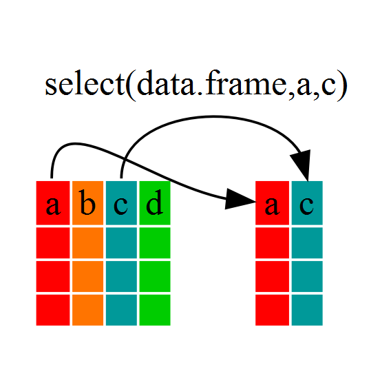
Using select()
If we wanted to use only a few of the variables in
our data frame we could use the select() function.
(Show diagram from “Challenges” page.)
year_country_gdp <- select(gapminder,year,country,gdpPercap)
year_country_gdp
Note that SQL has the same idea of select.
This is the normal R syntax, but the strength of dplyr lies in combining
several functions using pipes (like the bash shell). Since the pipes syntax
is unlike anything we’ve seen in R before, let’s repeat what we’ve done above
using pipes.
year_country_gdp <- gapminder %>% select(year,country,gdpPercap)
To help you understand why we wrote that in that way, let’s walk through it
step by step. First we summon the gapminder data frame and pass it on, using
the pipe symbol %>%, to the next step, which is the select() function.
In R, a pipe symbol is %>% while in the shell it is |.
Using filter()
We limit to European countries using select and filter.
year_country_gdp_euro <- gapminder %>%
    filter(continent=="Europe") %>%
    select(year,country,gdpPercap)
Line breaks between specific portions of our command make the code easier to read.
First we pass the data frame to filter then pass the filtered data frame to
select. Let’s reverse select and filter.
year_country_gdp_euro <- gapminder %>%
    select(year,country,gdpPercap) %>%
    filter(continent=="Europe")
1:57
Doesn’t work since we removed the continent column with select.
CHALLENGE 1: 5 min
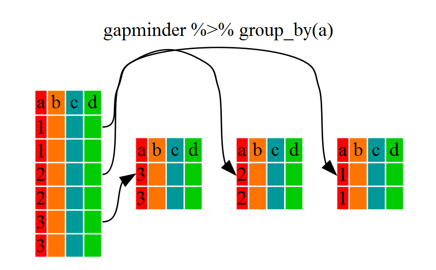
Using group_by() and summarize()
If you want to do this for each continent, you can reduce repetitiveness using
group_by. The function group_by is similar to filter.
str(gapminder)
str(gapminder %>% group_by(continent))
Notice that the structure of the data frame where we used group_by()
(grouped_df) is not the same as the original gapminder (data.frame).
Agrouped_df can be thought of as a list where each item in the listis a
data.frame which contains only the rows that correspond to a particular
value.
(Show diagram from “Challenges” page.)
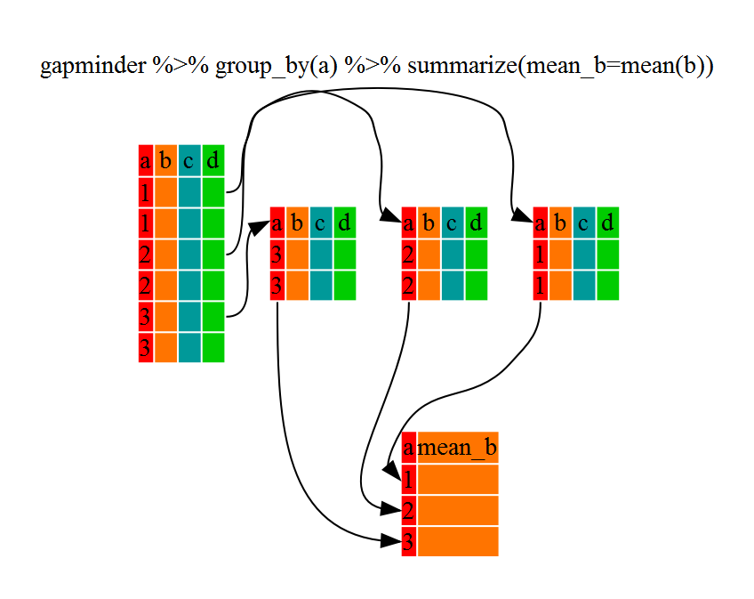
Using summarize()
group_by() is much more exciting in conjunction with summarize()
summarize allows us to create new variable(s) by using functions that repeat
for each of the continent-specific data frames.
gdp_bycontinents <- gapminder %>%
    group_by(continent) %>%
    summarize(mean_gdpPercap=mean(gdpPercap))
(Show diagram from “Challenges” page.)
2:11
That allowed us to calculate the mean gdpPercap for each continent, but it gets
even better.
CHALLENGE 2: 5 min
group_by() allows us to group by multiple variables. Let’s group by year
and continent.
gdp_bycontinents_byyear <- gapminder %>%
    group_by(continent,year) %>%
    summarize(mean_gdpPercap=mean(gdpPercap))
gdp_bycontinents_byyear
We can define more than 1 variable with summarize.
gdp_pop_bycontinents_byyear <- gapminder %>%
    group_by(continent,year) %>%
    summarize(mean_gdpPercap=mean(gdpPercap),
              sd_gdpPercap=sd(gdpPercap),
              mean_pop=mean(pop),
              sd_pop=sd(pop))
Using mutate()
We can create new variables prior to (or even after) summarizing information using mutate().
gdp_pop_bycontinents_byyear <- gapminder %>%
    mutate(gdp_billion=gdpPercap*pop/10^9) %>%
    group_by(continent,year) %>%
    summarize(mean_gdpPercap=mean(gdpPercap),
              sd_gdpPercap=sd(gdpPercap),
              mean_pop=mean(pop),
              sd_pop=sd(pop),
              mean_gdp_billion=mean(gdp_billion),
              sd_gdp_billion=sd(gdp_billion))
CHALLENGES 3 & 4: allot 10 min
Illustrate how to evaluate increasingly longer sections of a pipeline.
Coffee Break: 2:25–2:40
Creating Publication-Quality Graphics: 2:40–3:45
Plotting is one of the best ways to explore a dataset and the relationships between variables.
Today you’ll be using the ggplot2 package. It’s a bit harder to learn than
Base R plots but produces far higher quality.
(Ask them to get their ggplot2 cheat sheet.)
ggplot2 is built on the grammar of graphics (where the gg comes from):
the idea that any plot can be built from the same set of components:
- a data set
- a coordinate system
- a set of geoms—the visual representation of data points.
The key to understanding the grammar of graphics is thinking about a figure in layers (like Photoshop or Gimp).
Let’s start off with an example. The first thing we need to do is load the ggplot2 package.
library("ggplot2")
If you haven’t previously installed the package, install it now using the
command install.packages("ggplot2"). Then load it using the command above.
To begin graphing, we use the ggplot function. This lets R know that we’re
creating a new plot, and any of the arguments we give the ggplot function
are the global options for the plot: they apply to all layers on the plot.
ggplot(data = gapminder, aes(x = gdpPercap, y = lifeExp)) +
  geom_point()
Line breaks can be anywhere. The + is for another layer.

We’ve passed in two arguments to ggplot.
First, we tell ggplot what data we want to show on our figure (gapminder).
For the second argument we passed in the aes function, which
tells ggplot how variables in the data map to aesthetic properties of
the figure, in this case the x and y locations.
Here we told ggplot we want to plot the gdpPercap column of the gapminder
data frame on the x-axis, and the lifeExp column on the y-axis.
Other options that can be set with the aes function include color, size,
transparency and shape. We will talk more about that later.
By itself, the call to ggplot isn’t enough to draw a figure:
ggplot(data = gapminder, aes(x = gdpPercap, y = lifeExp))

We need to tell ggplot how we want to visually represent the data, which we
do by adding a new geom layer. In our example, we used geom_point, which
tells ggplot we want to visually represent the relationship between x and
y as a scatterplot of points:
2:56

CHALLENGES 1 & 2: 10 min
Layers
Using a scatterplot probably isn’t the best geom for visualizing change
over time. Instead, let’s tell ggplot to visualize the data as a line plot:
ggplot(data = gapminder, aes(x=year, y=lifeExp, by=country, color=continent)) +
  geom_line()

Instead of adding a geom_point layer, we’ve added a geom_line layer. We’ve
added the by aesthetic, which tells ggplot to draw a line for each
country. (This is another solution to Challenge 2.)
What if we want to visualize both lines and points on the plot? We can simply add another layer:
ggplot(data = gapminder, aes(x=year, y=lifeExp, by=country, color=continent)) +
  geom_line() + geom_point()

Like Photoshop, each layer is drawn on top of the previous layer. Here’s a slightly different version:
ggplot(data = gapminder, aes(x=year, y=lifeExp, by=country)) +
  geom_line(aes(color=continent)) + geom_point()

The aesthetic mapping of color has been moved from the global plot options in
ggplot to the geom_line layer so it no longer applies to the points.
Now we can clearly see that the points are drawn on top of the lines.
This changes the line color to red.
ggplot(data = gapminder, aes(x=year, y=lifeExp, by=country)) +
  geom_line(aes(color="red")) + geom_point()
Transformations and statistics
ggplot also makes it easy to overlay statistical models over the data. To
demonstrate we’ll go back to our first example:
ggplot(data = gapminder, aes(x = gdpPercap, y = lifeExp)) +
  geom_point()
3:12

It’s hard to see the mass of points on the left due to outliers “stretching” the x-scale.
You can change the scale of units on the x axis using the scale functions.
You can also modify the transparency of the points, using the alpha
function—that’s helpful when you have lots of data which is very clustered.
ggplot(data = gapminder, aes(x = gdpPercap, y = lifeExp)) +
  geom_point(alpha = 0.5) + scale_x_log10()

(Point out the logarithmic scale on the x-axis.) The alpha transparency allows
“additivity” of shading which wasn’t possible before.
The alpha aesthetic is applied only to geom_point. You can also make
transparency based on variables:
ggplot(data = gapminder, aes(x = gdpPercap, y = lifeExp)) +
  geom_point(aes(alpha = continent)) + scale_x_log10()
We can fit a least-square line to the data by adding another layer,
geom_smooth:
ggplot(data = gapminder, aes(x = gdpPercap, y = lifeExp)) +
  geom_point() + scale_x_log10() + geom_smooth(method="lm")

We can make the line thicker by setting the size aesthetic in the
geom_smooth layer:
ggplot(data = gapminder, aes(x = gdpPercap, y = lifeExp)) +
  geom_point() + scale_x_log10() + geom_smooth(method="lm", size=1.5)

Distinguish between the aesthetic alpha applying to a geom,
ggplot(data = gapminder, aes(x = gdpPercap, y = lifeExp)) +
  geom_point(alpha = 0.5)
i.e. alpha applies to all points, and alpha as a mapping between the data
and the points:
ggplot(data = gapminder, aes(x = gdpPercap, y = lifeExp)) +
  geom_point(aes(alpha = continent))
3:28
CHALLENGES 3 & 4: 10 min
Multi-panel figures
We can create a multi-panel figure this way:
starts.with <- substr(gapminder$country, start = 1, stop = 1)
az.countries <- gapminder[starts.with %in% c("A", "Z"), ]
ggplot(data = az.countries, aes(x = year, y = lifeExp, color=continent)) +
  geom_line() + facet_wrap( ~ country)

The facet_wrap layer takes a formula as its argument, denoted by the tilde
(~). This tells R to draw a panel for each unique value in the country column
of the gapminder dataset.
Modifying text
To clean up for publication, let’s rename our x and y axes using the xlab() and ylab() functions:
ggplot(data = az.countries, aes(x = year, y = lifeExp, color=continent)) +
  geom_line() + facet_wrap( ~ country) +
  xlab("Year") + ylab("Life Expectancy")

Now we give our figure a title with the ggtitle() function. And capitalize
the label of our legend. This can be done using the scales layer.
ggplot(data = az.countries, aes(x = year, y = lifeExp, color=continent)) +
  geom_line() + facet_wrap( ~ country) +
  xlab("Year") + ylab("Life Expectancy") +
  ggtitle("Figure 1") + scale_colour_discrete(name="Continent")

Let’s remove the x-axis labels so the plot is less cluttered. To do this, we
use the theme layer which controls the axis text and overall text size.
ggplot(data = az.countries, aes(x = year, y = lifeExp, color=continent)) +
  geom_line() + facet_wrap( ~ country) +
  xlab("Year") + ylab("Life Expectancy") +
  ggtitle("Figure 1") + scale_colour_discrete(name="Continent") +
  theme(axis.text.x=element_blank(), axis.ticks.x=element_blank())

Writing Data: 3:45–4:10
Saving plots
Making publication quality plots is great but does us little good if we cannot get them out of R and into our documents.
You can save a plot from within RStudio using the ‘Export’ button in the ‘Plot’ window

Writing data
At some point, you’ll also want to write out data from R.
We can use the write.table function for this.
Let’s create a data-cleaning script, for this analysis, we only want to focus on the gapminder data for Australia:
3:51
aust <- gapminder %>% filter(country == "Australia")
Before you write, use getwd() and setwd(...).
write.table(aust,          ## Gapminder data for countries located in Australia
  file="gapminder-aus.csv",## Name of the output file
  sep=","                  ## Comma separated
)
(Open terminal and cat this file.)
3:57
cat gapminder-aus.csv
head gapminder-aus.csv
You can also view the file by clicking on it in the Files tab.
Where did all these quotation marks come from? Also the row numbers are
meaningless. Let’s look at the help file for quote and row.names:
?write.table
By default R will wrap character vectors with quotation marks when writing out to file. It will also write out the row and column names.
4:03
write.table(aust,               ## Gapminder data for countries located in Australia
  file="gapminder-aus.csv",     ## Name of the output file
  sep=",",                      ## Comma separated
  quote=FALSE,                  ## Turn off quotation marks
  row.names=FALSE               ## No row names
)
Look at the data again in the Terminal tab.
head gapminder-aus.csv
That looks better!
CHALLENGE 1: 5 min
Wrap Up: 4:10–4:15
Help Files in R
Don’t forget your R helpfiles and package vignettes which can be accessed
by using the ? and vignette commands.
Supplemental Lessons
Additional R topics that we could not cover today.
RStudio cheat sheets
R quick reference guides including today’s handouts and more!
R for Data Science
Hadley Wickham is RStudio’s Chief Data Scientist and developer of the dplyr and ggplot2 packages.
R for Data Science is his newest book, and is available here for free.
One R Tip a Day on Twitter
Following One R Tip a Day is a great way to learn new tips and tricks in R.
Twotorials
Twotorials is a compilation of 2 minute youtube videos which highlight a specific topic in R.
Quick R Website
Cookbook for R
Advanced R
For more advanced topics, check out Hadley Wickham’s website based on his book “Advanced R”.
Remind them to fill out post-it survey